Polynomial ADTs & Moore
What's a polynomial functor, and how can they be used to represent finite state machines? With Scala's strong support for functional programming, and some guidance from Niu and Spivak, we can use polynomial functors to model our state machine in a type-safe and compositional way.

Table of Contents:
-
Introduction
-
Example: fs2 Stream Transducer
Introduction
Overview
Dependent lenses allow us to specify and manipulate state machines compositionally, using many of the familiar operations of polynomials.
Caveats and Goals
I'm not an expert in Poly. I'm a Scala developer, and a math enthusiast attempting to interpret aspects of Poly into Scala, a simply-typed programming language. As such, criticism is appreciated.
My goals here are:
- to explore the utility of a "lawless" implementation of a Poly in Scala, using ADTs and match types instead of fully dependent types
- to share and get feedback about this method of representing Poly, and the finite state machines they can model
- to try to make a Scala artifact out of the poly book, in the form of a library that can be improved over time
Background
Every category has its objects and its morphisms. The category of Poly consists of polynomial functors, and natural transformations from one polynomial functor to another.
Objects
The objects of Poly are polynomial functors. What's a polynomial functor? "... an arbitrary coproduct of representables". In Scala, we can model them using familiar algebraic data types (ADTs). How so?
The claim is that "Poly categorifies highschool math". If by "algebraic" we mean cardinality and the counting of values, and we do, then:
- An example provided in Haskell, y3 + y2 + 2:
data Foo y = Bar y y y | Baz y y | Qux | Quux - In Scala, we find
cats.data.Representable, and we can identify the methoddef index[A](f: F[A]): Representation => Aas a function that returns an exponential: ARepresentation, i.e., in polynomial format ofA => y, the term yA. - And when we look at the example of
cats.data.RepresentableStorewe can see thattype Store[S, A] =RepresentableStore[S => *, S, A]thus appears as a special case where both the functor and its indexing function are the same function,S => A, i.e., yS. Yet, note that neither coproducts norStorethemselves form aRepresentable(e.g., gist), and rather, as a sum of representables,Storeis a sum of anSnumber of representablesS => A, i.e.,S * (S => A), or, SyS.
So we can see how an ADT can be considered as a polynomial functor, for example, ByA:
sealed trait MyPolynomial[Y]
case class MyMonomial[A,B,Y](variable: A => Y, coefficient: B) extends MyPolynomial[Y]
And notably, we have the initial and terminal objects:
type `0`[Y] = MyMonomial[Nothing, Nothing, Y]
type `1`[Y] = MyMonomial[Unit, Nothing, Y]
Morphisms
"You'd never see, in highschool, arrows between polynomials, but they make sense". If the morphisms of Poly are maps from one polynomial functor to another, i.e., natural transformations, then can we model them in Scala? Yes, and no:
- On one hand, given types
P[_]andQ[_], then, thanks to Scala 3's polymorphic function types, it has never been easier to define a natural transformationval η: P ~> Q. - On the other hand, natural transformations in the full category of Poly are "dependent lenses", with
P ~> Qbeing "computed by Yoneda and the universal mapping-out property of coproducts". In other words, we'll need dependent functions in order to implement any natural transformation that is not a map between monomials. - In a future post we will explore some strategies for modelling the full range of polynomial morphisms in Scala 3. This post will focus on what we can implement with simple types: the full subcategory of Poly spanned by the monomials, a.k.a Jules Hedges' "bimorphic lenses".
The key to defining maps between polynomials is the pair of "view" and "update" functions, φ and φ#, required to implement their natural transformation. For example, take the two monomials mentioned above, cats.data.RepresentableStore (let's call it Store) and MyMonomial:
 /* Monomials p and q */
case class Store[S, Y](peek: S => Y, index: S)                   // Sy^S
case class MyMonomial[A, B, Y](variable: A => Y, coefficient: B) // By^A

/* A type alias, for natural transformations between p and q */
type ~>[F[_], G[_]] = [Y] =>> F[Y] => G[Y]

/* A "view" function, derived from the coefficients of p and q */
def φ: S => B

/* An "update" function, derived from the exponents of p and q */
def `φ#`: (S, A) => S

/* A natural transformation from p to q, formed by φ and φ# */
def η[S, A, B]: ([Y] =>> Store[S, Y]) ~> ([Y] =>> MyMonomial[A, B, Y]) =
  [Y] =>
    (store: Store[S, Y]) =>
      MyMonomial[A, B, Y](
        `φ#`.curried(store.index).andThen(store.peek),
        φ(store.index)
      )
Forgive the clunky type lambdas. In the polynomial morphism above, mapping one monomial to another, we can make use of the following observations:
- The pair of
viewandupdatefunctions completely specify the data of the natural transformation. - The polynomial that forms the codomain of the natural transformation can be said to "wrap" the polynomial that forms its domain.
In other words, monomial and polynomial morphisms are, respectively, simple and dependent lenses. And with type signatures like def ω: S𝑦S → B𝑦A, we can begin to see how to describe compositional state machines in the familiar language of polynomials. We'll be investigating the rich structure and the operations that this gives us access to.
Example: fs2 Stream Transducer
Let's look at polynomial functors in practice, beginning with the monomials: state lenses, wrappers, and wiring diagrams.


AB-Moore Machines
A poly map can model a Moore Machine. How so? Compare the above poly map between Store[S, Y] and MyMonomial[A, B, Y] to the definition of an AB-Moore machine, Moore[S, A, B], and note the similarity:
/* A "view" function */
def φ: S => B

/* An "update" function */
def `φ#`: (S, A) => S
/* A "view" function */
def get: S => B

/* An "update" function */
def put: (S, A) => S

/* An "initial value" function */
def init: SAs we build bigger and more complex machines, we'll see that Moore machines compose nicely and have their role. However there is one feature that a Moore machine lacks: a run function. And, for that, we turn to Mealy machines.
AB-Mealy Machines
A poly map can also model a Mealy Machine. An AB-Mealy Machine is essentially a Moore machine with a run function, i.e., an ABA-Moore Machine. That is, given a value of the state, the machine outputs a "B", but the "B" is a function A => B, so that type Mealy[S, A, B] =
Moore[S, A, A => B]. This let's us implement a run function, forming a finite state machine ideal for stream processing. Note the similarity between the run function and the argument to the mapAccumulate function as we'd find in cats or fs2:
/* A "view" function */
def φ: S => A => B

/* An "update" function */
def `φ#`: (S, A) => S

/* A "run" function */
def run: (S, A) => (S, B) =
    (s, a) =>
(`φ#`(s, a), φ(s)(a))/* A stream transducer function */
def transducer[F[_], S, A, B](
fsm: Moore[S, A, A => B]
): fs2.Stream[F, A] => fs2.Stream[F, B] =
stream =>
stream
.mapAccumulate(fsm.init)(
(s, a) =>
(fsm.put(s, a), fsm.get(s)(a)))
.map(_._2)
So, starting from two data types, Store[S, Y] and MyMonomial[A, B, Y], we've arrived at a simple state machine with a standardized run function. From this we can conclude:
- Simple types are sufficient for modeling maps between monomials, and the state machines they represent.
- Given a state,
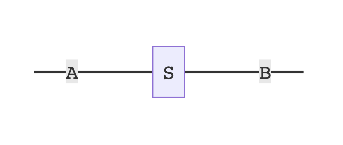
S, and an interface, referred to here asA ‒⛶→ B, we can form a map from one to the other, yielding a dynamical systemA ‒🅂→ B. - View and update functions, and their types, are derived mechanically from the two functors, in a manner specified by the natural transformation of the two functors.
Once the init, readout, and update functions are provided, and a behavior of the state machine is thereby defined, then we have a Mealy machine, ready to process data:
val m: Moore[Monomial.Store[Boolean, _] ~> Monomial.Interface[Int, Int => Int, _]] =
  Moore[Boolean, Int, Int => Int, Y](
    false,
    s => x => if s then x + x else x,   // if we've seen x > 1, then emit 2x
    (s, x) => if x > 1 then true else s // change state upon seeing x > 1
  )

val n: Mealy[Monomial.Store[Boolean, _] ~> Monomial.Interface[Int, Int => Int, _]]
  m.asMealy

val l: List[Int] =
  List(1, 2, 3).mapAccumulate(n.init)(n.run)._2
// l: List[Int] = List(1, 2, 6)
Wiring Diagrams
Sometimes we care only about wires. That is, the interaction patterns alone, with the stateful components abstracted away, to be composed at a later step.
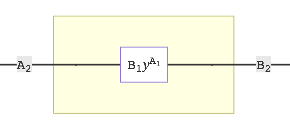
In the polynomial maps discussed so far, we've seen that if given a state, S, and an interface, referred to here as A ‒⛶→ B, we can form a map from one to the other, yielding a dynamical system A ‒🅂→ B. But poly maps can also represent wiring diagrams and enclosures, like -[‒A‒⛶‒B‒]-, where there is a "hole" for the state lens, and each box is an interface.
When a wiring diagram is composed with a state system, the outermost interface of the composite lens is called the "wrapper interface", where it serves as an adaptor to modify the state lens:
extension [S, A1, B1, Y] (p: (Store[S, _] ~> Interface[A1, B1, _])[Y])
  def andThen[A2, B2](
    w: (Interface[A1, B1, _] ~> Interface[A2, B2, _])[Y]
  ): (Store[S, _] ~> Interface[A1, B1, _] ~> Interface[A2, B2, _], _])[Y] =
    new (Store[S, _] ~>  Interface[A1, B1, _] ~> Interface[A2, B2, _])[Y]:
      def φ: PolyMap.Phi[Store[S, _] ~>  Interface[A1, B1, _], Interface[A2, B2, _], Y] =
        p.φ.andThen(w.φ)
      def `φ#`: PolyMap.PhiSharp[Store[S, _] ~>  Interface[A1, B1, _], Interface[A2, B2, _], Y] =
        (s, a) => p.`φ#`(s, w.`φ#`(p.φ(s), a))
We should quickly note some points about using Scala's simple types instead of fully dependent types:
- We incur some library boilerplate by using simple types instead of dependent types.
- We use match types
PhiandPhiSharpfor three purposes: to mitigate boilerplate, to derive function types, and to abstract over arity. - Hidden there in the Greek is the familiar, loopy, "there and back" implementation of lens composition.
But the main point is that, through lens composition, we've used a wiring diagram to turn an unrunnable Moore machine into a runnable Mealy machine. Once we initialize it and provide view and update functions, then we're ready for data:
val l: Moore[Store[Boolean, _] ~> Interface[Int, Int, _]] =
  Moore(false, s => if s then 1 else 0, (s, i) => s)

val m: Mealy[Store[Boolean, _] ~> Interface[Int, Int, _] ~> Interface[Int, Int => Int, _]] =
  l.andThen(Wiring(i => j => j + j, (i1, i2) => i2)).asMealy

val l: List[Int] =
  List(1, 2, 3).mapAccumulate(m.init)((s, i) => m.run(s, i))._2
// List(2, 4, 6)A satisfying result. But this is only the beginning, it seems. We'll end this post having seen only monomials and only the most basic lenses. In order to see all that Poly has to offer, we'll need to explore a little further, and see just how far we can get with Scala's simple types.
Other posts in this series:
References
- https://topos.site/poly-book.pdf
- https://youtu.be/7ZaL6aQVOZo
- https://github.com/tpolecat/tpolecat.github.io/blob/master/presentations/algebraic_types.html
- https://youtu.be/3AOGDTr1zrY
- https://www.youtube.com/live/GswIAurBIYY
- https://youtu.be/U-W7GT0BUTU
- https://blog.oyanglul.us/scala/dotty/en/functionk
- https://github.com/julianpeeters/dynamical
- https://github.com/julianpeeters/polynomial
- https://gist.github.com/julianpeeters/9e02d0342db41d286f91e02f24617b7a
- https://gvolpe.com/blog/fsm-fs2-a-match-made-in-heaven/